ㅊKeras로 신경망을 작성하는 절차
model = tf.models.Sequential()
model.add(tf.keras.layers.Dense(units=2, input=(2,), activation='sigmoid'))
model.add(tf.keras.layers.Dense(units=1, activation='sigmoid'))
model.compile(loss='mean_squared_error', optimizer=keras.optimizers.SGD(lr=0.3))
model.fit(X, y, batch_size=1, epochs=10000)
print(model.predict(X))
compile(optimizer, loss=None, metrics=None) : 훈련을 위해서 모델을 구성하는 메소드
fit(x=None, y=None, batch_size=None, epochs=1, verbose=1) : 훈련 메소드
evaluate(x=None, y=None) : 테스트 모드에서 모델의 손실 함수값과 측정 항목 값을 반환
predict(x, batch_size=None) : 입력 샘플에 대한 예측값을 생성
add(layer) : 레이어를 모델에 추가
Keras 사용 방법
1) Sequential 모델을 만들고 모델에 필요한 레이어를 1 추가하는 방법
model = Sequential()
model.add(Dense(units=2, input_shape=(2, ), activation='sigmoid'))
model.add(Dense(units=1, activation='sigmoid'))

2) Sequential 모델을 만들고 모델에 필요한 레이어를 추가하는 방법
model = Sequential()
model.add(Dense(units=2, input_shape=(2, ), activation='sigmoid'))
model.add(Dense(units=3, activation='sigmoid'))
model.add(Dense(units=1, activation='sigmoid'))


keras의 클래스들
- 모델 : 하나의 신경망을 나타낸다
- 레이어 : 신경망에서 하나의 층
- 입력 데이터 : 텐서플로우 텐서 형식
- 손실 함수 : 신경망의 출력과 정답 레이블 간의 차이를 측정하는 함수
- 옵티마이저 : 학습을 수행하는 최적화 알고리즘. 학습률과 모멘텀을 동적으로 변경한다.
Input(shape, batch_size, name) : 입력을 받아서 케라스 텐서를 생성하는 객체
Dense(units, activation=None, use_bias=True, input_shape) : 유닛들이 전부 연결된 레이어
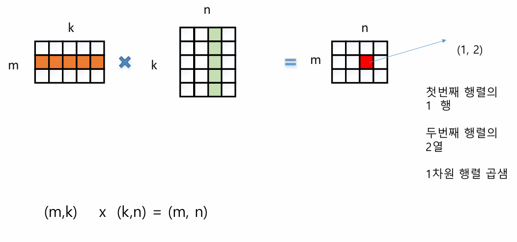
tf.keras.layers.Dense
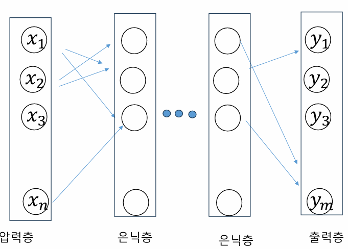
완전 연결 계층 : 한 층의 모든 뉴런이 그 다음 층의 모든 뉴런과 연결된 상태

케라스 신경망 파라미터 -loss (손실 함수)
- 회귀
- MeanSquaredError : 정답 레이블과 예측값 사이의 평균 제곱 오차를 계산
- 분류에 사용되기도 함
- 분류
- BinaryCrossentropy : 정답 레이블과 예측 레이블 간의 교차 엔트로피 손실을 계산한다
ex) 강아지, 강아지 아님
- CatrgoryCrossentropy : 정갑 레이블과 예측 레이블 간의 교차 엔트로피 손실을 계산한다.
ex) 강아지, 고양이, 호랑이. (정답 레이블은 원핫 인코딩으로 제공되어야 한다)
- SparseCategoricalCrossentropy : 정답 레이블과 예측 레이블 간의 교차 엔트로피 손실을 계산한다.
ex) 강아지, 고양이, 호랑이. (정답 레이블은 정수로 제공되어야 한다)
One hot encoding
3개의 class 강아지, 고양이, 호랑이 일 때, 한개의 1과 복수의 0으로 이루어진 벡터로 표현
- 강아지 (0) => 1, 0, 0
- 고양이 (1) => 0, 1, 0
- 호랑이 (2) => 0, 0, 1
-

from tensorflow import keras
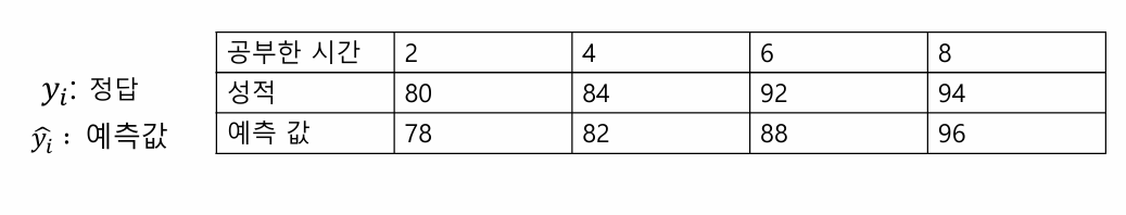
y_true = [80, 84, 92, 94]
y_pred = [70, 80, 90, 100]
mse=keras.losses.MSE
print(mse(y_true, y_pred).numpy())

from tensorflow import keras
y_true = [1, 0, 0, 1]
y_pred = [0.7, 0.2, 0.3, 0.9]
bce = keras.losses.BinaryCrossentropy()
print(bce(y_true, y_pred).numpy())
from tensorflow import keras
y_true = [1, 0, 0, 1]
y_pred = [0.6, 0.3, 0.4, 0.7]
bce = keras.losses.BinaryCrossentropy()
print(bce(y_true, y_pred).numpy())

from tensorflow import keras
y_true = [[0, 1, 0], [0, 0, 1], [1, 0, 0]]
y_pred = [[0.6, 0.3, 0.1], [0.3, 0.6, 0.1], [0.7, 0.1, 0.2]]
cce = keras.losses.CategoricalCrossentropy()
print(cce(y_true, y_pred).numpy())
from tensorflow import keras
y_true = [[0, 1, 0], [0, 0, 1], [1, 0, 0]]
y_pred = [[0.9, 0.0, 0.1], [0.2, 0.7, 0.1], [0.8, 0.1, 0.1]]
cce = keras.losses.CategoricalCrossentropy()
print(cce(y_true, y_pred).numpy())
keras 신경망 파라미터 : batch_size
- 샘플을 몇 개 사용하여 가중치를 변경할 지 단위
- batch_size가 너무 크면 학습 속도가 느려지고,
- 너무 작으렴 학습 과정이 불안정해질 수 있음
- 변수 (w, b)가 업데이트 되는 단위
1 epoch는 전체 샘플이 처리되는 기준
전체 샘플이 300개이고, batch_size가 30이면, 1 epoch동안 10번 가중치가 update됨
전체 샘플이 300개이고, batch_size가 10이면, 1 epoch동안 30번 가중치가 update됨
Metric : 측정 항목
Accuracy : 정확도. 예측값이 정답 레이블과 같은 횟수를 계산한다
MeanSquaredError : MSE
넘파이 배열
TensorFlow Dataset 객체 : 크기가 커서, 메모리에 한번에 적재될 수 없는 경우에 디스크 또는 분산 파일 시스템에서 스트리밍 될 수 있다.
파이썬 제너레이터 :

import matplotlib.pyplot as plt
import tensorflow as tf
(train_images, train_labels), (test_images, test_labels) = tf.keras.datasets.mnist.load_data()
print(train_images.shape)
print(train_labels)
print(test_images.shape)
plt.imshow(train_images[0], cmap="Greys")
model = tf.keras.models.Sequential()
model.add(tf.keras.layers.Dense(512, activation='relu', input_shape=(784,)))
model.add(tf.keras.layers.Dense(10, activation='sigmoid'))
model.compile(optimizer='rmsprop',
loss='mse',
metrics=['accuracy'])
train_images = train_images.reshape((60000, 784))
train_images = train_images.astype('float32') / 255.0
test_images = test_images.reshape((10000, 784))
test_images = test_images.astype('float32') / 255.0
train_labels = tf.keras.utils.to_categorical(train_labels)
test_labels = tf.keras.utils.to_categorical(test_labels)
model.fit(train_images, train_labels, epochs=5, batch_size=256)
test_loss, test_acc = model.evaluate(test_images, test_labels)
print('테스트 정확도:', test_acc)
plt.show()

핵심 포인트
유닛 수가 커질수록, 배치 사이즈가 작아질 수록 정확도는 올라간다!
하지만 학습 속도가 느려질 가능성이 있다..
범주형 데이터 처리

정수 인코딩
sklearn 라이브러리가 제공하는 Label Encoder 클래스를 사용
import numpy as np
X = np.array([['Korea', 44, 7200],
['Japan', 27, 4800],
['China', 30, 6100]])
from sklearn.preprocessing import LabelEncoder
labelencoder = LabelEncoder()
X[:, 0] = labelencoder.fit_transform(X[:, 0])
print(X)
[['2' '44' '7200']
['1' '27' '4800']
['0' '30' '6100']]
import numpy as np
X=np.array([['Korea', 44, 7200],
['Japan', 27, 4800],
['China', 30, 6100]]) # Removed extra space before this line
from sklearn.preprocessing import OneHotEncoder # Added a missing space
onehotencoder= OneHotEncoder()
# 원하는열을뽑아서2차원배열로만들어서전달하여야한다.
XX = onehotencoder.fit_transform(X[:,0].reshape(-1,1)).toarray()
print(XX)
X = np.delete(X, [0], axis=1) # 0번째열삭제
X = np.concatenate((XX, X), axis = 1) # X와XX를붙인다.
print(X)
[[0. 0. 1.]
[0. 1. 0.]
[1. 0. 0.]]
[['0.0' '0.0' '1.0' '44' '7200']
['0.0' '1.0' '0.0' '27' '4800']
['1.0' '0.0' '0.0' '30' '6100']]
원 핫 인코딩
import numpy as np
X = np.array(['Korea', 'Japan', 'China'])
from sklearn.preprocessing import OneHotEncoder
onehotencoder = OneHotEncoder()
XX = onehotencoder.fit_transform(X.reshape(-1, 1)).toarray()
print(XX)
[[0. 0. 1.]
[0. 1. 0.]
[1. 0. 0.]]
케라스의 to_catetorical()
class_vector = [2, 6, 6, 1]
from tensorflow.keras.utils import to_categorical
output = to_categorical(class_vector, num_classes=7)
print(output)
[[0. 0. 1. 0. 0. 0. 0.]
[0. 0. 0. 0. 0. 0. 1.]
[0. 0. 0. 0. 0. 0. 1.]
[0. 1. 0. 0. 0. 0. 0.]]

아래 문자열 입력을 정수형으로 변경하고 print하는 code를 작성하시오
import numpy as np
X = np.array(['apple','grape','melon','orange'])
from sklearn.preprocessing import LabelEncoder
labelencoder = LabelEncoder()
XX = labelencoder.fit_transform(X)
print(XX)
[0 1 2 3]
아래 문자열 입력을 원 핫 인코딩으로 변경하고 print하는 code를 작성하시오.
import numpy as np
X = np.array(['apple','grape','melon','orange'])
from sklearn.preprocessing import OneHotEncoder
onehotencoder = OneHotEncoder()
XX = onehotencoder.fit_transform(X.reshape(-1, 1)).toarray()
print(XX)
[[1. 0. 0. 0.][0. 1. 0. 0.] [0. 0. 1. 0.] [0. 0. 0. 1.]]
아래 class vector를 원 핫 인코딩으로 변경하고 print하는 code를 작성하시오.
from tensorflow import keras
class_vector =[8, 3, 2, 5]
from tensorflow.keras.utils import to_categorical
output = to_categorical(class_vector, num_classes=10)
print(output)
[[0. 0. 0. 0. 0. 0. 0. 0. 1. 0.]
[0. 0. 0. 1. 0. 0. 0. 0. 0. 0.]
[0. 0. 1. 0. 0. 0. 0. 0. 0. 0.]
[0. 0. 0. 0. 0. 1. 0. 0. 0. 0.]]
케라스 딥러닝 - 소프트 맥스
총헙아 1안 형태로 변환

케라스 신경망 실습 - 패션 아이템 분류
- 이미지는 28*28 크기
- 픽셀 값은 0과 255 사이
- 레이블은 0부터 9 까지


model = models.Sequential()
model.add(layers.Flatten(input_shape=(28, 28)))
model.add(layers.Dense(32, activation='relu'))
model.add(layers.Dense(10, activation='softmax'))
model = models.Sequential()
model.add(layers.Flatten(input_shape=(28, 28)))
model.add(layers.Dense(64, activation='relu'))
model.add(layers.Dense(16, activation='relu'))
model.add(layers.Dense(10, activation='softmax'))

판다스
- 데이터를 머신러닝이나 시각화에 적절하도록 전처리 해주는 라이브러리
- 자료구조 : 데이터 프레임
- import pandas as pd


케라스 신경망 실습 - 타이타닉 생존자 예측
PassengerId : 각 승객의고유번호
Survived : 생존 여부(종속변수) •0 = 사망 •1 = 생존
Pclass : 객실 등급-승객의사회적, 경제적지위 •1st = Upper •2nd = Middle •3rd = Lower
Name : 이름 Sex : 성별 Age : 나이
SibSp : 동반한Sibling(형제자매)와
Spouse(배우자)의수 Parch : 동반한
Parent(부모) Child(자식)의 수
Ticket : 티켓의 고유넘버
Fare : 티켓의 요금
Cabin : 객실 번호
Embarked : 승선한 항 •C = Cherbourg •Q = Queenstown •S = Southampton
import numpy as np
import pandas as pd
import tensorflow as tf
# 데이터 세트를 읽어들인다.
train = pd.read_csv("train.csv", sep=',')
test = pd.read_csv("test.csv", sep=',')
# 필요없는 컬럼을 삭제한다.
train.drop(['SibSp', 'Parch', 'Ticket', 'Embarked', 'Name',\
'Cabin', 'PassengerId', 'Fare', 'Age'], inplace=True, axis=1)
test.drop(['SibSp', 'Parch', 'Ticket', 'Embarked', 'Name',\
'Cabin', 'PassengerId', 'Fare', 'Age'], inplace=True, axis=1)
# 결손치가 있는 데이터 행은 삭제한다.
train.dropna(inplace=True)
test.dropna(inplace=True)
# 기호를 수치로 변환한다.
for ix in train.index:
if train.loc[ix, 'Sex']=="male":
train.loc[ix, 'Sex']=1
else:
train.loc[ix, 'Sex']=0
for ix in test.index:
if test.loc[ix, 'Sex']=="male":
test.loc[ix, 'Sex']=1
else:
test.loc[ix, 'Sex']=0
# 2차원 배열을 1차원 배열로 평탄화한다.
target = np.ravel(train.Survived)
# 생존여부를 학습 데이터에서 삭제한다.
train.drop(['Survived'], inplace=True, axis=1)
train = train.astype(float) # 최근 소스에서는 float형태로 형변환하여야
test = test.astype(float) # 최근 소스에서는 float형태로 형변환하여야
# 케라스 모델을 생성한다.
model = tf.keras.models.Sequential()
model.add(tf.keras.layers.Dense(16, activation='relu', input_shape=(2,)))
model.add(tf.keras.layers.Dense(8, activation='relu'))
model.add(tf.keras.layers.Dense(1, activation='sigmoid'))
# 케라스 모델을 컴파일한다.
model.compile(loss='binary_crossentropy',
optimizer='adam',
metrics=['accuracy'])
# 케라스 모델을 학습시킨다.
model.fit(train, target, epochs=30, batch_size=1, verbose=1)

model = tf.keras.models.Sequential()
model.add(tf.keras.layers.Dense(16, activation='relu', input_shape=(2,)))
model.add(tf.keras.layers.Dense(8, activation='relu'))
model.add(tf.keras.layers.Dense(8, activation='relu'))
model.add(tf.keras.layers.Dense(1, activation='sigmoid'))
0.7436
model = tf.keras.models.Sequential()
model.add(tf.keras.layers.Dense(16, activation='relu', input_shape=(2,)))
model.add(tf.keras.layers.Dense(16, activation='relu'))
model.add(tf.keras.layers.Dense(8, activation='relu'))
model.add(tf.keras.layers.Dense(1, activation='sigmoid'))
0.8120